How to Detect Anomalies in Time Series for Enterprise AI

To detect anomalies in time series, start by defining what an "anomaly" means for the business. This is not just a technical exercise; it's about translating a statistical deviation into a business event, such as a drop in user sign-ups or a spike in server latency that precedes an outage.

Defining the business problem is the first and most critical step. It dictates the data you collect, the models you choose, and how you measure success.

Defining What Anomaly Detection Solves for Your Business

Before writing code, answer one question: what specific problem are we trying to solve?

Without a clear business purpose, you risk building a system that flags statistically interesting but operationally irrelevant events. I have seen teams build models that generate thousands of alerts, none of which mattered to the business. This leads to alert fatigue and shelved projects.

Draw a direct line from a technical anomaly to a business outcome. A 30% increase in API error rates is not just a number; it is a potential customer-facing outage that can reduce revenue and damage brand reputation.

Anomaly detection is not about finding statistical outliers. It is about identifying events that threaten operational stability, financial health, or the customer experience. The goal is to build a system that produces actionable alerts.

Classifying Anomalies by Business Impact

Classify anomalies based on their shape and the business scenario they represent. Each type suggests a different problem and often requires a unique detection strategy.

Categorizing them provides a common language between data science and operations teams. Here is a breakdown of the main types you will encounter.

<br>

Types of Time Series Anomalies and Business Scenarios

Anomaly Type	Definition	Enterprise Example (Healthcare)	Enterprise Example (Finance)
Point Anomaly	A single data point that deviates from the rest of the series.	A sudden, extreme spike in a patient's heart rate monitor, indicating a potential cardiac event.	A single, large withdrawal from a bank account inconsistent with the customer's transaction history.
Contextual Anomaly	A data point that is abnormal only within a specific context, like time of day.	A surge in emergency room admissions for respiratory issues on a day with low air pollution levels.	A spike in retail stock trading volume at midnight, when markets are typically closed.
Collective Anomaly	A sequence of data points that are not individually anomalous but are unusual as a group.	A gradual, sustained decline in patient oxygen saturation levels over an hour, signaling developing respiratory distress.	A series of small, rapid transactions across multiple accounts, which together form a money laundering pattern.

<br>

Thinking in these terms helps move from a vague "something's wrong" to a specific, classifiable event your model can be trained to recognize.

Setting Clear and Measurable Goals

Once you know what an anomaly looks like, set concrete, quantifiable goals. This aligns business and technical teams and helps prove ROI. Avoid vague goals like "improve monitoring."

A well-defined project goal might look like one of these examples:

• Reduce manufacturing equipment failures by 8% to 15% from the Q2 baseline by detecting subtle deviations in sensor data before they become critical.
• Decrease false positive fraud alerts by 20% to free up the security team's time to focus on high-risk investigations.
• Improve system uptime by proactively flagging server health issues, with a target of a 10% reduction in P1 incidents per quarter.

This level of precision ensures everyone is aligned. For example, financial teams can see how detecting unusual stock volume and trading breakouts directly impacts trading strategies. Framing your project with these kinds of goals turns it from a technical experiment into a strategic business initiative.

Before proceeding, it is useful to assess your current readiness by completing a project audit. Find out more at https://dsg.ai/audit.

Preparing and Engineering Data for Anomaly Detection

The foundation of an effective anomaly detection model is the data, not the algorithm. In enterprise systems, raw time series data is rarely ready for use. It often contains missing values, noise, and irregular timestamps that can mislead models.

Addressing these data quality issues is fundamental. A model fed with noisy, incomplete data will produce unreliable alerts, eroding trust and rendering the system ineffective.

Handling Missing Data and Noise

The first task is often dealing with gaps in your data. Missing points can result from network issues in an IoT sensor or a brief server outage. Your strategy for filling these gaps must match the data's behavior.

For metrics that change gradually, like daily active users, linear interpolation is a reasonable choice. For more volatile data, where the last known value is the best predictor of the next, a forward-fill approach is often more appropriate.

Once gaps are filled, you must address the noise. System metrics can be volatile, making it difficult to distinguish a real anomaly from random fluctuations. A moving average can smooth the data and reveal the underlying trend. If your data has strong seasonal patterns, exponential smoothing is more effective, as it gives more weight to recent data points.

Be cautious not to over-smooth your data, as this can obscure the anomalies you are trying to find. The goal is to reduce meaningless noise, not flatten the entire signal. Start with a small smoothing window, such as a 3-point moving average, and increase it only if necessary.

The Power of Feature Engineering

With a clean dataset, the next step is feature engineering. This involves creating new variables from your time series that provide the model with important context. This step often has the greatest impact on model performance.

Good feature engineering transforms a simple stream of numbers into a multi-dimensional view, making it easier for a model to learn the pattern of "normal" behavior.

Creating Temporal and Statistical Features

You can create powerful features by examining the data's history and statistical properties. Three types of features consistently deliver useful results:

• Lag Features: These are values from previous time steps—the value from an hour ago, a day ago, or a week ago. They help the model understand momentum and recurring patterns.
• Rolling Statistics: Calculating statistics over a moving window gives your model a dynamic baseline for what is currently normal. A 7-day rolling standard deviation can highlight recent volatility, while a 24-hour rolling average helps define typical behavior for a specific time of day.
• Calendar-Based Features: Context is important. Adding features like the day of the week, hour of the day, or flags for holidays changes the model's understanding. A large spike in e-commerce traffic is expected on Black Friday, but the same spike on a Tuesday in April is an anomaly.

Here is a Python example using the pandas library to show how to create these features. This synthetic example assumes you have a DataFrame df with a timestamp index and a 'value' column.

# Synthetic data example
import pandas as pd
import numpy as np

# Create a sample DataFrame
rng = pd.date_range('2023-01-01', periods=100, freq='D')
df = pd.DataFrame({'value': np.random.randint(0, 50, size=(100))}, index=rng)

# 1. Lag Features
df['lag_1_day'] = df['value'].shift(1)
df['lag_7_day'] = df['value'].shift(7)

# 2. Rolling Statistics
df['rolling_mean_7_day'] = df['value'].rolling(window=7).mean()
df['rolling_std_7_day'] = df['value'].rolling(window=7).std()

# 3. Calendar-Based Features
df['day_of_week'] = df.index.dayofweek # Monday=0, Sunday=6
df['is_weekend'] = df['day_of_week'].isin([5, 6]).astype(int)

print(df.head(10))

By engineering these features, you provide the model with a rich, contextual understanding of the data, which it needs to detect anomalies in time series data with precision.

Picking the Right Anomaly Detection Method

When it comes to detecting anomalies in time series data, there is no single best algorithm. The choice depends on your data's characteristics, whether you have historical examples of anomalies, and your latency requirements. You will need to balance simplicity against the ability to spot complex patterns.

This field has grown significantly. A review of research papers from 2014 to 2024 shows a 500% increase in publications. The main drivers are cybersecurity (35% of studies), finance (25%), and healthcare (20%). The trend is a shift from simple statistical methods to machine learning, with unsupervised models now accounting for 60% of all published techniques. You can find more details in this decade-long analysis of anomaly detection research on arxiv.org.

This shift reflects the complexity of enterprise data. We can group the methods into three categories: statistical, classic machine learning, and deep learning.

Statistical Methods: Your First Line of Defense

Statistical methods are foundational to anomaly detection and are often the best starting point. If your time series is predictable with stable averages or consistent seasonal cycles, these techniques can be effective. Their main advantages are simplicity and transparency; when an anomaly is flagged, the reason is clear.

Two established and useful options include:

• Z-Score or Modified Z-Score: This method measures how far a data point deviates from the average. It is fast and works well for data that follows a normal distribution. The modified version, which uses the median instead of the mean, is less affected by the outliers you are trying to find.
• Seasonal Hybrid ESD (Extreme Studentized Deviate): This technique is suitable for data with strong seasonal patterns, like weekly sales or daily website traffic. It decomposes the time series into its trend and seasonal components before searching for outliers.

These methods have low computational requirements and provide a solid baseline. Their limitation is that they can be confused by complex data with shifting underlying patterns.

Classic Machine Learning: Finding Unknowns Without Labels

When you do not have labeled examples of anomalies, unsupervised machine learning is a practical choice. Instead of being trained on what an anomaly looks like, these models learn the pattern of "normal" behavior and flag anything that does not conform. This makes them suitable for detecting novel problems.

In practice, unsupervised learning is often the most practical approach. Manually labeling data is slow and expensive. Furthermore, the most dangerous anomalies are often unexpected. These models are designed to find "unknown unknowns."

Two common unsupervised models are:

• Isolation Forest: This algorithm is based on the principle that anomalies are rare and different, making them easy to isolate. It is efficient and can handle large datasets.
• One-Class SVM (Support Vector Machine): This model builds a boundary around the normal data. Any data point that falls outside this boundary is flagged as an anomaly. It is particularly useful for high-dimensional feature spaces.

These models offer a significant advantage over statistical methods for more complex patterns without requiring labeled data.

Deep Learning: For When Things Get Really Complicated

For the most challenging time series—those with complex, non-linear relationships and long-term dependencies—deep learning models can provide higher accuracy. They can detect subtle signals that other methods might miss. However, this power comes with higher computational costs and can be difficult to interpret (the "black box" problem).

Key deep learning models include:

• LSTMs (Long Short-Term Memory networks): As a type of recurrent neural network (RNN), LSTMs are effective at modeling sequences. You can train an LSTM to predict the next step in a time series. When the prediction is significantly different from the actual value, it likely indicates an anomaly.
• Autoencoders: This is a type of unsupervised neural network that learns to compress data into a lower-dimensional representation (encode) and then reconstruct it (decode). When trained on normal data, it becomes proficient at this reconstruction. When presented with an anomaly, it struggles, resulting in a high "reconstruction error" that serves as an anomaly signal.

To help you navigate these choices, here is a summary of the trade-offs.

Comparison of Anomaly Detection Methods

This table outlines the core differences between the main approaches, helping you match the right technique to your team's needs, resources, and data.

Method	Best For	Computational Cost	Interpretability	Requires Labeled Data?
Statistical	Stable data with clear seasonality or trends.	Low	High	No
Classic ML	Complex data with few or no labeled anomalies.	Medium	Medium	No (Unsupervised)
Deep Learning	Highly complex, non-linear patterns.	High	Low	Optional (Can be Supervised or Unsupervised)

Choosing the right method is a balance between performance, the business problem, and operational constraints. A practical strategy is to start with a simpler model, like a statistical or classic ML method, and only use deep learning if the additional performance is necessary.

How to Evaluate Your Model and Set Alerting Thresholds That Actually Work

You have built a model. The next step is evaluation and thresholding, which determines if your system will be a useful tool or an ignored nuisance. A model's value is in the alerts it generates.

A common pitfall is using standard classification metrics. Anomalies are rare by definition. If only 0.1% of your data is anomalous, a model that always predicts "normal" will achieve 99.9% accuracy but will be useless.

Picking Metrics That Matter for Imbalanced Data

To accurately measure performance when you detect anomalies in time series data, you must use metrics designed for imbalanced datasets. The most common are Precision, Recall, and the F1-score, which are derived from the confusion matrix.

Let's reframe the confusion matrix for this problem:

• True Positives (TP): The model correctly flagged a real anomaly.
• True Negatives (TN): The model correctly ignored a normal data point.
• False Positives (FP): The model flagged a normal point as an anomaly (a false alarm).
• False Negatives (FN): The model missed a real anomaly (a critical failure).

With this framework, we can focus on metrics that provide useful information.

Precision answers the question: "Of all the alerts we received, how many were actually real?" (TP / (TP + FP)). High precision means fewer false alarms. Recall asks: "Of all the real anomalies that occurred, how many did we catch?" (TP / (TP + FN)). High recall means fewer missed critical events.

You will find a trade-off between Precision and Recall. Increasing sensitivity to catch more anomalies (improving recall) will likely lead to more false alarms (lowering precision). The F1-score (2 * (Precision * Recall) / (Precision + Recall)) provides a single, balanced measure of a model's effectiveness.

The Art and Science of Setting Thresholds

The threshold determines whether a model's anomaly score triggers an alert. Setting this value is critical for the system's usability. A threshold that is too sensitive will generate a high volume of alerts that get ignored. A threshold that is too lenient will miss important events.

This is a business decision, not just a statistical one. You need to discuss the costs with stakeholders.

• In a payment processing system, a missed anomaly (false negative) could result in significant financial loss from fraud. In this case, you would tolerate more false alarms to maximize recall.
• For monitoring a non-critical internal application, the cost of a false positive—such as waking an engineer at 3 AM—is likely higher than the impact of a few minutes of degraded performance.

A useful tactic is to use dynamic thresholds instead of static ones. For example, you could set the threshold based on the rolling 99th percentile of anomaly scores from the previous 24 hours. This allows the system to adapt to natural variations, like a holiday traffic spike, without triggering unnecessary alerts.

As you fine-tune these systems, it is important to have a structured framework for measuring their performance and business value. For a deeper look into this process, you can learn more about how to assess and validate AI systems. Finding the right balance is an iterative process that requires testing, communication with business teams, and an understanding of the operational impact of each alert.

Getting Your Anomaly Detection System Ready for the Real World

Moving a time series anomaly detection model from a development environment to a live production system is a significant undertaking. A good F1-score is not enough if the system cannot deliver reliable, low-latency results 24/7. This transition requires a robust architecture for data processing, model serving, and ongoing maintenance.

A production-ready system must be resilient and trustworthy. Deploying the model is only one part of the process. You also need a strong governance framework to monitor its behavior, manage its lifecycle, and ensure it complies with company standards and regulations.

Building Scalable Deployment Pipelines

First, you need to automate the entire workflow. The goal is to build a pipeline that handles everything from data ingestion and feature engineering to real-time model inference. To detect anomalies in time series data as they happen, a streaming architecture is necessary.

This type of setup usually includes several core components:

• Real-Time Data Ingestion: You need a system that can handle a high volume of data from sources like IoT sensors or application logs. Tools such as Apache Kafka or AWS Kinesis are designed for this purpose.
• Model Serving: The model must be accessible via a low-latency API endpoint. The industry standard is to use Docker for containerization and Kubernetes for orchestration to ensure scalability and resilience.
• Latency Requirements: The business use case determines the required speed. A fraud detection system might need a response in under 50 milliseconds, while a system monitoring factory equipment could have a few seconds. This requirement will influence your choice of model and infrastructure.

The objective is an automated system that can ingest new data, get a prediction from the model, and send an alert without manual intervention. For more information on building these automated workflows, you can explore enterprise-grade AI orchestration and automation.

Monitoring for Model and Concept Drift

An anomaly detection model requires ongoing monitoring. The environment and your data change over time. This phenomenon, known as concept drift, means a model trained on last year's data may become outdated as user behavior or market conditions shift.

Continuous monitoring is essential. You should track not only the model's predictions but also the statistical properties of the incoming data. A significant shift in the data's mean or variance is a strong indicator that the model's definition of "normal" is no longer accurate.

A sudden drop in model performance or a gradual increase in the number of alerts often indicates concept drift. A practical approach is to set up automated triggers to retrain the model whenever its F1-score degrades by a predetermined amount, such as 10% from its baseline.

This cycle of proactive monitoring and retraining is necessary to maintain the long-term accuracy and value of your system.

The infographic below illustrates the ongoing process of assessing data, balancing risks, and setting appropriate alert thresholds, which is a critical part of managing the system.

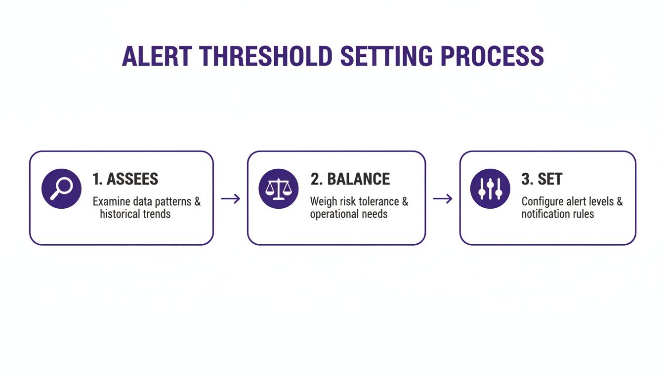
As this guide shows, setting alerts is a continuous loop of evaluation and adjustment to maintain system effectiveness.

Ensuring AI Governance and Compliance

As AI becomes more integrated into business operations, governance and compliance are now essential. Regulations like the EU AI Act impose strict requirements for transparency, explainability, and risk management, especially for high-risk systems.

An effective governance framework provides the necessary controls for your AI. It should include:

• Audit Trails: Every prediction, alert, and retraining job must be logged. This creates a complete history that is valuable for debugging and demonstrating compliance.
• Explainability: In many situations, flagging an anomaly is not enough. Stakeholders will want to know why a data point was flagged. Techniques like SHAP (SHapley Additive exPlanations) can provide this context.
• Risk Management: You need a formal process to identify and mitigate risks, which can range from model bias to security vulnerabilities.

The value of these systems is evident in fields like public health. An analysis of historical mortality data from France found that 1.27% of observations were anomalies corresponding to major wars and epidemics. During the COVID-19 pandemic, similar methods identified mortality spikes 5-10 times higher than normal in certain weeks. For businesses, this same capability can flag a dangerous change in a patient's vital signs or a surge in hospital admissions, helping teams respond proactively.

Platforms like DSG.AI's manageAI Monitoring and assureIQ are designed to provide these governance capabilities, helping you ensure your AI systems are powerful, responsible, compliant, and ready for the enterprise.

Frequently Asked Questions About Time Series Anomaly Detection

As teams implement anomaly detection systems, several common questions arise. The transition from theory to a live production environment presents consistent challenges. Here are some of the most frequent questions we hear from enterprise teams.

Should I Use a Supervised or Unsupervised Approach?

This decision depends on your data. If you have a large amount of high-quality, labeled data where every past anomaly is identified, a supervised approach can be effective. It learns directly from these historical examples. However, this is uncommon.

In most cases, teams have little to no labeled anomaly data. This is where an unsupervised approach is most useful. Models like Isolation Forest or Autoencoders are designed for this scenario. They learn the pattern of "normal" behavior from your data and then flag any deviations. This makes them suitable for detecting new or unexpected anomalies, which is essential for applications like cybersecurity, fraud detection, or system health monitoring.

What's the Single Biggest Challenge in Deploying an Anomaly Detection System?

The biggest challenge is balancing the detection of genuine problems (true positives) with the generation of false alarms (false positives). This balance is controlled by the detection threshold.

Setting this threshold is both a science and an art. If it is too low, you will miss critical events. If it is too high, you will overwhelm your operations team with irrelevant alerts, leading to "alert fatigue," where even real warnings are ignored.

The key is to frame the problem in terms of business impact. Discuss with stakeholders the cost of a missed event versus the cost of investigating a false alarm. This conversation will help you set a threshold that aligns with business goals and your team's capacity.

How Often Should I Retrain My Model?

You should retrain your model when the data indicates it is necessary, not on a fixed schedule. The key factor to monitor is concept drift. This occurs when the underlying patterns in your data change over time due to shifts in user behavior, process updates, or market dynamics. When this happens, your model's definition of "normal" becomes obsolete.

To manage concept drift, you need a monitoring plan that tracks two things:

• Model Performance: Monitor metrics like the F1-score. A sustained drop, such as a 10% degradation from your baseline, is a clear signal to retrain.
• Data Distribution: Monitor the statistical properties of your incoming data, like its mean and variance. A significant shift indicates that the real-world environment has changed and your model may no longer be relevant.

This data-driven approach ensures you retrain only when necessary, saving computational resources while maintaining system accuracy.

Can This Actually Work in Real-Time?

Yes. Real-time detection is the primary goal for many critical applications, such as financial fraud prevention and IoT sensor monitoring. However, it requires a more sophisticated architecture than batch processing.

A real-time system needs several components working together:

1. A Streaming Data Pipeline: A system like Apache Kafka is needed to handle a continuous flow of data.
2. A Low-Latency Model Endpoint: The model must be served as a fast, scalable API that can respond in near real-time.
3. An Efficient Alerting Mechanism: When an anomaly is detected, alerts must be sent within seconds.

Your choice of model is also important. For real-time applications, lighter-weight models like Isolation Forest or a pre-trained Autoencoder are often preferred. They can provide predictions quickly, helping to meet strict latency requirements, which are often under 100 milliseconds.

---

At DSG.AI, we specialize in designing and deploying enterprise-grade AI systems that deliver measurable business value. Our architecture-first approach ensures your anomaly detection solutions are scalable, reliable, and seamlessly integrated into your existing workflows. We turn your data into a competitive advantage. Explore our real-world projects to see how.